Running Models

A simulation is run in one of two ways. For both ways, a Java Runtime Environment is required as is the Scala Build Tool. sbt is used to run the simulation.

Pre-packaged models

If the model is in some sense “finished” and has been published to one of the standard binary class repositores such as Maven Central, no extra software is necessary to run it, only the .properties file that instructs sbt where to get it is needed. An example .properties file looks like this. It can then be downloaded and run like so:

% sbt @mois-examples.properties
Getting uk.ac.ed.inf mois-examples_2.11 1.99.3-SNAPSHOT ...
downloading ...
...
Error: Must specify a command
mois 1.99.3-SNAPSHOT
Usage: mois [info|list|model] <args>...

Command: info <model>
Get information on a model
  <model>
        Model name

Command: list
List models

Command: model [options] <model>
Run a model
  -d <value> | --duration <value>
        Simulation duration (mandatory)
  -b <value> | --begin <value>
        Simulation start time (default: 0.0)
  -i <value> | --initial <value>
        Initial conditions filename (JSON)
  -s <value> | --state <value>
        Dump state at end of simulation
  -o <value> | --output <value>
        Output specification
  <model>
        Model name

Allowed output specifications:
	gui[:vars...]		Simple plot to a graphical window.
	netcdf:<file>		NetCDF output to the given file
	png:<file>[:vars...]	Simple plot to a PNG file
	tsv			Tab-separated values to standard output
	tsv:<file>		Tab-separated values to the given file

The helpful message displayed says that you must tell the program what to do! At the time of writing, three commands are supported.

• list prints a list of available models
• info takes a model as argument and prints out detailed information about it
• model runs the model and requires at least a --duration

Let’s go ahead and try these.

% sbt @mois-examples.properties list
Known models:
	uk.ac.ed.inf.mois.examples.BollenbachModel
	uk.ac.ed.inf.mois.examples.HénonModel
	uk.ac.ed.inf.mois.examples.PendulumModel
	uk.ac.ed.inf.mois.examples.PySpiralModel
	uk.ac.ed.inf.mois.examples.RoesslerModel
	uk.ac.ed.inf.mois.examples.SampleODEModel

Suppose we would like more information about the Pendulum model. It isn’t necessary to type out the whole long name, just enough to make it unambiguous (“Pe” would be minimally sufficient in this case, but “P” would not because it would also match the python spiral model”:

% sbt @mois-examples.properties info Pendulum
model parameters:
    Double(p0) := -10.0
    Int(n) := 41
    Double(θ0) := 0.0
    Double(p_delta) := 0.5
    Double(m) := 1.0
    Double(l) := 1.0
process tree:
            mass: 1.0
            type: Hamiltonian
          length: 1.0
            name: Pendulum
   mois-examples: 1.99.3-SNAPSHOT
           title: Planar Pendulum
           class: uk.ac.ed.inf.mois.examples.Pendulum
            mois: 1.99.3-SNAPSHOT
       variables:
          Double(y) := -1.0
                           units: m
                       long_name: Y position in cartesian coordinates
          Double(E) := 0.0
                           units: J
                       long_name: Total energy
          Double(θ) := 0.0
                           units: rad
                       long_name: Angle anti-clockwise from vertically downwards
          Double(x) := 0.0
                           units: m
                       long_name: X position in cartesian coordinates
          Double(p) := 0.0
                           units: J.s
                       long_name: Angular momentum

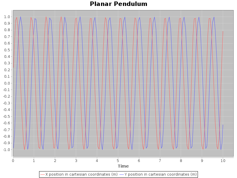
To actually run a model, and show a graph of the last few datapoints for the x and y variables during execution, or alternatively write a plot out as an image, one could then do

% sbt @mois-examples.properties model --duration 10 -o gui:x,y Pendulum
% sbt @mois-examples.properties model --duration 10 \
    -o png:pendulum-xy.png Pendulum

Which produces this image:

Developing and Modifying Models

The other way is to obtain a copy of the source code for the examples, and run sbt on its own. From the interactive shell it is possible to simply use the run command, with arguments as above:

% git clone https://github.com/edinburgh-rbm/mois-examples.git
% cd mois-examples
% sbt 
> run model --duration 1 --output gui Pendulum
[info] Updating {file:.../mois-examples/}mois-examples...
[info] Resolving jline#jline;2.11 ...
[info] Done updating.
[info] Compiling 4 Scala sources to .../mois-examples/target/scala-2.11/classes...
[info] Running uk.ac.ed.inf.mois.MoisMain model --duration 10 --output gui Pendulum
[success] Total time: 5 s, completed Jul 8, 2014 10:53:57 PM
>

This way of running the simulation is useful while the model is being developed because it will automatically recompile any source code files that have been changed before actually running.